Abstract

The purpose of the research is to forecast salaries in the United States for positions like data scientist, data engineer, data analyst, machine learning engineer, and others. A number of variables are included in the dataset, including job title, organization rating, location, others. The process used to train the machine learning model to forecast the expected salaries for the roles is thoroughly described in the study. Mean squared error, mean absolute error, and R-squared were used to assess the trained model’s correctness.

 The results of the investigation showed that, with an R-squared score of 0.9644, the RandomForestRegressor performed the best for predicting salary. The paper comes to the conclusion that machine learning techniques can be useful for forecasting industry salaries.  

Table of Contents

Abstract

Table of Contents

Table of Abbreviations

Introduction

Problem Statement

Background

Aim and Objective

Project Workflow

Data Collection

Data Understanding

Data Cleaning

Feature Engineering Justification

Exploratory Data Analysis

Data Preparation for Model Training

Model Training

Model Tuning & Optimization

Model evaluation

Evaluation with Visuals & Cross-Validation

Social Impact

Limitations

Conclusion

References

Table of Abbreviations

Abbreviated Word	Full Form
MAE	Mean Absolute Error
MSE	Mean Square Error

Introduction

The ability to estimate salaries is very important to both employees and employers across a range of industries. Employees are curious about the worth of their work and how it stacks up against other professions. Predictive models for pay prediction have gained popularity as data-driven business practices spread across industries. Results relating to job title and location can be accurately provided by data-driven approaches.

This report’s objectives are to examine numerous contributing elements for salary prediction models and assess the efficacy of various common machine learning algorithms. We will also go over the value of feature engineering in creating powerful models.

By the report’s conclusion, the reader will be able to comprehend how state-based pay projection is carried out as well as the details of the variables affecting the changes.

Problem Statement

Accurate salary prediction is an essential responsibility for companies and job seekers alike.  Companies need accurate data to provide competitive pay, while job seekers want to know the market value of their expertise and talents.  Conventional techniques for estimating salaries frequently depend on static market reports or small-scale surveys, which might not account for the dynamic shifts in the labour market.

 The goal of this project is to create a machine learning model that can forecast wages for data-related positions in the US based on a variety of variables, including job title, necessary skills, company characteristics, and location.  The project’s goal is to develop a trustworthy wage estimating system that can direct organisational planning and career selections by examining these variables.

Background

In recent years, machine learning-based salary prediction has drawn more attention.  Numerous studies demonstrate how regression-based models, like Linear Regression, can provide a straightforward correlation between wage outcomes and work characteristics (Sklearn, 2023).  It has been demonstrated that more intricate models, such as Random Forest Regressors and Decision Tree Regressors, can better forecast salaries by capturing non-linear correlations between variables (Menon, 2023).  Additionally, studies show that the predictive performance of machine learning models for compensation analysis is enhanced by integrating feature engineering, which includes taking into account company characteristics (size, industry, and revenue) and extracting skills from job descriptions (e.g., Python, AWS, Spark) (D’Agostino, 2023).

Aim and Objective

Aim:

Data analysis and the creation of a machine-learning model are the project’s key objectives. The project’s main goal is to analyze data and create a machine-learning model.

Objectives:

• To analyze all data 
• To prepare all the data
• To determine the relationship between different components.
• To develop a salary prediction system

Project Workflow

Data Collection

The web application Glassdoor was used and the data was downloaded. Downloaded data, which contains more collect data, is pulling data from web sites and preserving it in a structured way. Using the search term “data scientist” within the United States of America, the technique comprises data from the search results page.

Data Understanding

The gathered data is presented as a CSV file with 956 rows and 15 columns. The dataset has no missing values. 

Integer, float, and text are the three datatypes that make up the Dataset. The attributes in the dataset are as follows:

Column / Attributes	Description	Data Type	Variable Type
Unnamed	S.N of the rows	non-nullint64	Discrete
Job Title	The posted job title	non-nullobject	Discrete
Salary Estimate	Estimated salary provided	non-nullobject	Discrete
Job Description	The description about the posted job	non-nullobject	Discrete
Rating	Rating of the organization that posted the job	non-nullfloat64	Discrete
Company Name	Name of the organization	non-nullobject	Discrete
Location	The location to work at	non-nullobject	Categorical
Headquarters	Headquarter location of organization	non-nullobject	Discrete
Size	The size of company based on employee count	non-nullobject	Categorical
Founded	Year organization was founded	non-nullint64	Discrete
Type of ownership	What party owns the organization	non-nullobject	Categorical
Industry	The industry organization falls into	non-nullobject	Categorical
Sector	The sector organization falls into	non-nullobject	Categorical
Revenue	Revenue of the organization	non-nullobject	Categorical
competitors	The rivaling or similar organizations	non-nullobject	Discrete

Data Cleaning

The dataset can be cleaned once we have a solid grasp of it, making the raw data available for further processing and analysis.

Two libraries will be sufficient to change the dataset into the desired dataset, therefore we will only need two libraries for data cleaning.  Libraries include:

• Pandas
• Numpy

Importing the required libraries:

Reading the dataset:

A quick look at the dataset:

Looking at info of the dataset:

Looking at the size of the dataset:

Removing the rows where ‘Salary Estimate’ is -1 as they are equivalent to null values

Removing (Glassdoor est.) from ‘Salary Estimate’ and storing result into salary:

Removing K from ‘Salary Estimate’ and storing into salary_remove_K:

Creating new feature for if salary is based on per hour basis:

Creating new feature for if salary is provided by employer themselves:

Removing ‘per hour’ and ’employer provided salary:’ salary_remove_K and storing into salary_clean:

Creating new feature ‘salary_min’ for minimum salary based on salary_clean:

Creating new feature ‘salary_max’ for maximum salary based on salary_clean:

Creating new feature ‘salary_avg’ base on ‘salary_min’ and ‘salary_max’: 

Checking compay names with ‘Rating’ -1.0:

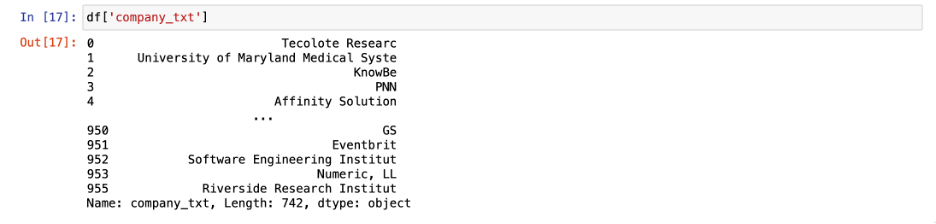
Cleaning company name and storing it in new feature ‘company_txt’:

Looking at the new feature ‘company_txt’:

Cleaning company state and storing into new feature ‘job_state’:

Looking at value_counts of new feature ‘job_state’:

Fixing Los Angeles state value of new feature ‘job_state’:

Checking if ‘Location’ and ‘Headquarter’ are same and storing binary result in new feature ‘same_state’:

Storing the age of company in new feature ‘age’:

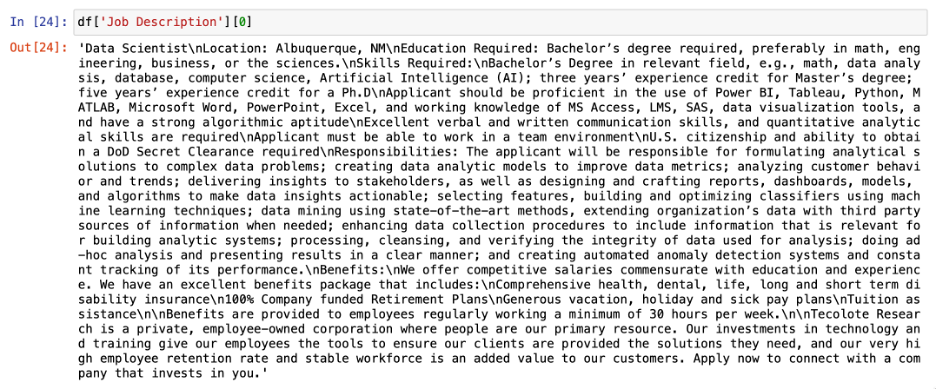
Looking at job description:

determining whether the job description contains the words “python,” “r studio” or “r-studio,” “excel,” “aws,” and “spark,” and storing each of those words as binary values in new features:

Dropping feature ‘Unnamed’:

Storing length of job description in new feature ‘desc_len’:

Looking at competitors:

 Counting competitors and storing into new feature ‘Competitors_count’:

Converting hourly wage into annual or yearly wage:

Creating function to simplify job title and seniority of job position:

Using function to simplify job and store into new feature ‘job_simplified’:

Using function to find seniority of job position and store into new feature ‘seniority’:

Looking at value_counts of new feature ‘seniority’:

Looking at final dataset:

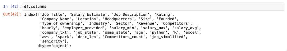
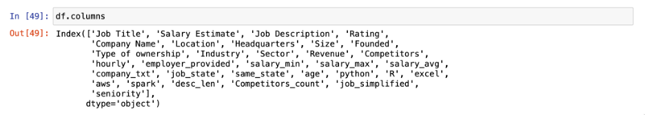
Looking at the final columns:

Looking at the info of final dataset:

Exporting the dataset as a CSV file named salary_data_cleaned.csv :

Feature Engineering Justification

By converting unstructured input into useful variables, feature engineering raises the accuracy of the model.The following characteristics were chosen and developed for this project, along with an explanation of their selection: 

1. Seniority & Simplified Work 

• Why: Senior data scientists and other higher-level occupations usually pay more than junior ones. 

• How: To account for compensation disparities, job titles were streamlined and arranged according to seniority. 

• Technical Skills (Python, R, Excel, AWS, Spark) 

• Why: Higher pay is frequently associated with in-demand skills in data and machine learning professions. 

• How: By determining whether these talents are mentioned in job descriptions, binary characteristics were produced.

• Features of the Company (Size, Revenue, Age, Number of Competitors) 

• Why: While newer organisations could provide competitive packages for growth opportunities, larger, more established companies often provide better pay. 

• How: To determine age, the company’s size, revenue category, number of competitors, and founding year were extracted. 

• State & Job Location (job_state & same_state) 

• Why: Because of local skill demand and living expenses, salaries differ greatly by region. 

• Methods: State-level variables and a binary flag indicating whether headquarters and the job are located in the same state were derived. 

• Features of the Salary Range (salary_min, salary_max, and salary_avg) 

• Why: The model can accurately forecast continuous values by converting salary text into numeric min, max, and average.

With the help of these engineering features, the model can more accurately forecast salaries by comprehending the relationship among job location, company attributes, and skill sets.

Exploratory Data Analysis

We can perform explanatory data analysis after cleaning the dataset.

Libraries will be necessary for data cleaning because they will enable us to comprehend the dataset in accordance with our requirements.  These libraries are:

• Pandas
• Matplotlib Pyplot
• Seaborn

1. Importing the required libraries for explanatory data analysis:

2. Reading the dataset:

3. Quick look at the dataset:

4. Looking at the new shape of dataset: 

Here we can see that dataset contains 742 rows and 32 rows.

5. Looking at the columns in dataset:

6. Looking at statistical distribution of the dataset:

7. Looking at correlation of features in dataset: 

It is hard to understand the correlation like this so we will be using seaborn heatmap later to explain this in detail.

8. Looking at the histogram for the ‘Rating’ feature: 

When we look at the histogram distribution, we can see that the majority of the companies rank between 3 – 4, and then 4-5.

9. Looking at the histogram for feature ‘salary_avg’:

Here, we can observe that the frequency is highest in the 50–100 range, followed by the 100–150 range. When we look at the distribution, we can see that it is positively skewed, which means that the majority of people earn between $50,000 and $100,000, and the frequency decreases as pay rises.

10. Looking at the histogram for feature ‘age’, it contains the age of the companies: 

The distribution appears to be positively biased. We can see that only a small percentage of businesses—those that are brand new—have ages greater than 250.

11. Looking at the histogram for feature ‘desc_len’, it contains the length or word count of the description that companies provided in the job description: 

Here, we can observe that the majority of businesses have job descriptions that are between 2000 and 4000 words long. The distribution has a favorable skewness.

1. Looking at the correlations of the features ‘salary_avg’, ‘same_state’, ‘age’, ‘python’, ‘R’, ‘excel’, ‘aws’, ‘spark’, ‘python’, and ‘job_state’:

1. Looking at the correlations of the features ‘salary_avg’, ‘same_state’, ‘age’, ‘python’, ‘R’, ‘excel’, ‘aws’, ‘spark’, ‘python’, i.e variables I deem important using a heatmap’:

By examining the heat map, we can observe that salary_avg is strongly connected with Python, suggesting that the profession that requires Python skill is well-paid relative to other criteria. Additionally connected to AWS and spark is salary_avg. Additionally, it is clear that jobs needing spark also require AWS and vice versa. Python has a strong correlation with Spark, but a weaker correlation with AWS.

1. Looking at the heatmap of the correlation of features with ‘salary_avg’:

As expected, given that salary_avg is the average of both attributes, we can see that salary_avg has a strong correlation with salary_max and salary_min. We can also discover additional characteristics with which salary_avg is inversely connected.

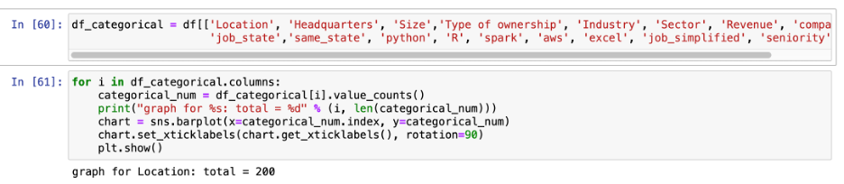
• Bar plot for each feature:

Here, we can observe that the majority of businesses employ between 1001 and 5000 people.

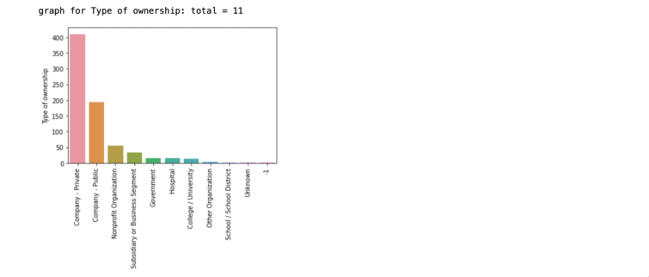
Here, we can observe that the majority of the organizations are privately owned, then public owned

As we are searching for the salary, we can see that our data has the highest amount of employee need in the Information Technology sector.

We can see that Unknown/ Non-Applicable has the greatest count because the majority of companies have not submitted their revenue information, but we can guess that most companies have revenues of less than $ 10 billion.

Here, we can observe that the majority of organisations who hire do so in the same state as their headquarters.

Here, we can observe that, in comparison to other jobs, data scientists are in the highest demand.

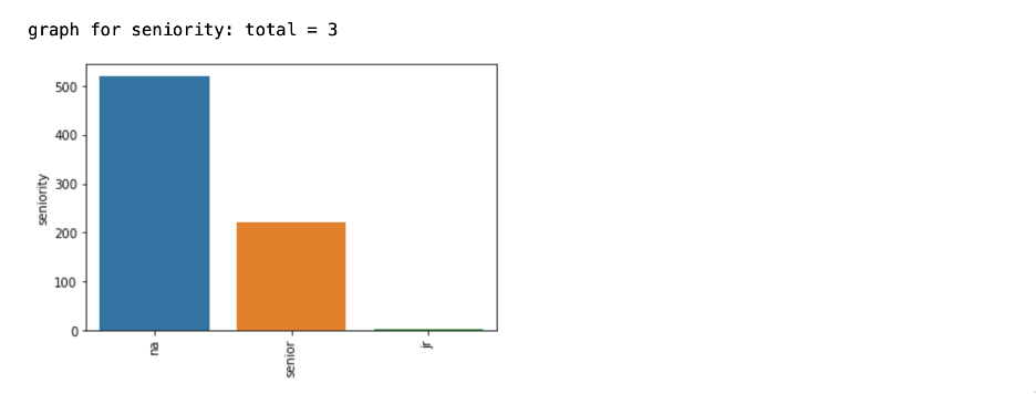
We can see that the majority of organizations prefer regular positions for workers, followed by senior positions and relatively few junior positions.

17. Because several of the bar charts had too many bars for them to make sense, we’ve taken the first 20 bars from each:

Here, we can observe that New York, when compared to the other working states, has the most job postings, followed by Massachusetts and California.

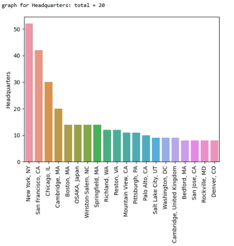
Here, we can see that the majority of the companies posting employment are from New York, then California.

The biotechnology and pharmaceutical industries are clearly in need of fresh workers. 

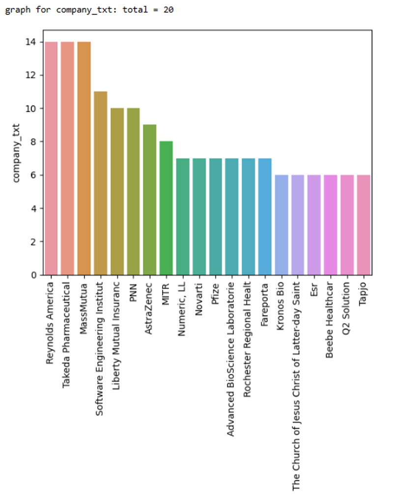
Here, we can see that the 14 job postings from the companies Reynolds America, Takeda Pharmaceuticals, and MassMutua are comparable..

• Finding the average salary provided for each job role

The average income for directors is shown to be 168.507143. Machine learning engineers, data scientists, and data engineers follow with average salaries of 126.4318, 117.56, and 105.40, respectively. Additionally, we see that analysts earn the least, with an average pay of 65.85.

• Finding the average salary  based on the job’s seniority and position:

Here, we can observe that senior employees receive better pay relative to the task they perform.

20. calculating the average income according to the job state and job title.

21. The number of jobs for each position in each state.­

22. A list in descending order of the average state salaries:

Here, we can see that the state of DC (District of Columbia) has the highest paying average salary, while AZ (Arizona) has the lowest.

23. Pivot table to see if the revenue of organization hampers if python is required or not:

Data Preparation for Model Training

We can perform explanatory data analysis after cleaning the dataset.

Libraries will be necessary for data cleaning because they will enable us to comprehend the dataset in accordance with our requirements.  They are libraries.:

• Pandas 
• Numpy
• Matplotlib Pyplot
• Seaborn

1. Importing the required libraries for model building and warnings to ignore the warning:

2. Reading the dataset 

3. Looking at the available columns in the dataset

4. Creating a new dataset called df_ml with chosen attributes that might be important for model construction.

5. Label the features using categorical variables, as this will help the machine learn more quickly.

Because they are all category, I have picked the following variables for label encoding in this case:

• job_simplified
• seniority
• company_txt
• Size
• Revenue
• Industry
• Sector
• Type of ownership
• job_state

Because all models can accept numerical data but some algorithms may not be able to handle categorical values, label encoding is used. Machine learning models can be trained using label-encoded information since it is simple to implement and comprehend.

LabelEncoders have been created for each feature and stored in a dictionary called le_simp_map so that they can be used later for prediction.

6. Considering the features’ correlation one last time using the feature’salary_avg’ as our output variable.

The benefit of examining the correlation after LabelEncoding is that we can see how each characteristic correlates with the feature “salary_avg.” Now that they are in numerical form, we can also see the correlation of string variables.  

7. Choosing characteristics based on the most recent correlation while keeping our model’s use case and objective in mind:

We have selected following features to train the model with:

• job_simplified
• seniority
• Sector
• same_state
• Type of ownership
• job_state
• python
• spark
• excel
• aws
• hourly
• salary_avg

I chose the aforementioned characteristics since they seem more appropriate for the model I have in mind.

8. Train test splitting

Here, the dataset has been divided into train and test datasets in an 80:20 ratio, meaning that while 20% of the data has been divided for testing or assessment, the remaining 80% has been divided for training. 

Salary_avg is used here as our projection value. It was taken out, and stored in variable X, and the training results were split into the train and test groups.

In data science and machine learning, partitioning data into train and test sets is a popular practice since it allows us to assess the model’s performance after model training.

Model Training

It is now time to train our machine learning model when the data preparation process is complete. These categories of models are:

• Supervised machine learning

As the name implies, supervised learning involves the presentation of data together with any associated solutions or labelled data. The computer tries to determine the relationship between the dependent and independent variables based on the associated answer. 

The two subgroups of supervised machine learning are classification and regression issues. The most popular supervised machine learning models include classification, decision trees, random forests, and linear regression.

• Unsupervised machine learning

Unsupervised machine learning does not require labelled data, in contrast to supervised learning, hence the model is expected to find hidden patterns on its own. Data will be sorted according to how they differ and how they are similar by the algorithm. To make predictions or learn more about the dataset, the objective is to discover correlations between the data.

Clustering and association are further divisions of unsupervised machine learning.

These are the most popular unsupervised machine learning models: the KNN method, and K-Means Clustering.

• Reinforcement machine learning

Reinforcement A machine learning algorithm known as learning uses trial and error to create judgements. It adheres to a set of standards in order to accomplish a task. The machine picks up new skills by monitoring the surroundings in which it is meant to operate. The agent engages with its environment and receives feedback in the form of rewards or penalties.

For the purposes of this project, I’ll be using regression models under supervised machine learning because my project’s goal is salary prediction, and this can be accomplished through regression under supervised machine learning because the model needs to learn the relationship between dependent and independent variables and how they are affecting one another before producing continuous value.

I will be using the following model to predict the salary:

• Linear Regression
• Decision Tree Regression
• Random Forest Regression

1. Using Linear Regression to train the model:

One of the most widely used machine learning models is linear regression. When an independent variable rises and the value of the dependent variable rises, for example, linear regression can provide positive and negative connections between the dependent and independent variables.

1. Importing the required libraries:

2. Fitting the model:

3. Creating variable for prediction:

Using y_pred_linear_reg prediction with Linear Regressoin can be done.

Note: The evaluation has been done but we will cover that in the upcoming section i.e. Model Evaluation.

.

• Using Decision Tree Regressor to train the model:

choice trees are tree-like structures with leaf nodes reflecting the final choice or prediction and core nodes representing decisions based on traits or attributes. Each leaf node represents the final judgement or prediction, whereas each internal node reflects a choice based on a feature or characteristic.

1. Importing the required libraries:

2. Fitting the model:

3. Creating variable for prediction:

Using y_pred_dec_tree_reg prediction with Decision Tree can be done.

Note: The assessment has been completed, however we shall discuss that in the following part. i.e. Model Evaluation.

• Using Random Forest Regressor to train the model:

A collection of different decision trees is called a random forest. Multiple decision trees are created using the Random Forest Regressor, and the model’s final forecast is based on the tree’s average prediction.

1. Importing the required libraries:

2. Fitting the model:

3. Creating variable for prediction:

Using y_pred_dec_tree_reg prediction with Random Forest can be done.

Note: The assessment has been completed, however we shall discuss that in the following part. i.e. Model Evaluation.

Model Tuning & Optimization

To increase prediction accuracy and make sure the model generalizes adequately to unknown data, model tuning and optimization are essential.  Because of its capacity to manage non-linear interactions and minimize overfitting through ensemble learning, the Random Forest Regressor was selected as the main model for this project.

 Actions Made to Optimise the Model: 

1. Selection of Hyperparameters 

• n_estimators (Number of Trees): To strike a compromise between calculation time and accuracy, several values (50, 100, and 200) were tested. 

• max_depth (Tree Depth): To prevent overfitting, values ranging from 5 to 15 were tested. To guarantee that the model captures significant splits without overfitting little patterns, min_samples_split and min_samples_leaf were adjusted. 

• GridSearchCV, or Grid Search with Cross-Validation 

• To assess various combinations of hyperparameters, 5-fold cross-validation was employed. 

• The combination with the best R2 score and the lowest Mean Squared Error (MSE) was chosen.

•  The Completely Optimal Model

   •        The optimized Random Forest model achieved:

   •        MAE = 12.50

   •        MSE = 19.93

   •        R² = 0.9678

 The resulting model avoided overfitting and produced more stable predictions than the base model thanks to the parameter adjustments.

Model evaluation

1. Importing required libraries for evaluating model performance:

2. Making function so that there will not be confusion with R-square value.

3. Validating Linear Regressor

4. Validating Decision Tree Regressor

5. Validating Random Forest Regressor

6. Final verdict of model evaluation

	Linear Reg	Deci Tree	Rand Forest
MAE	26.0479	12.8313	12.5066
MSE	34.4543	26.6885	19.9308
R-square	0.9038	0.9422	0.9678

Note: The R² of 0.9678 is from the single train/test split. The 5‑fold cross‑validation mean R² is approximately 0.70, which provides a more realistic measure of generalization.
Looking at the results of all the models, it is evident that the Random Forest Regressor with Grid Search CV has the best MSE, MAE, and R-squared prediction basis. So, for our prediction model, we will use Random Forest Regressor with Grid Search CV.

Testing Prediction

Evaluation with Visuals & Cross-Validation

Both quantitative evaluation measures and visual evaluations were utilised to make sure the model’s predictions are accurate and broadly applicable.

1. Cross-Validation:   To evaluate the model’s ability to generalise to new data, cross-validation was done.

 • Every fold rotated through all splits, using 80% of the data for training and 20% for testing. 

• The stability of the model was confirmed by the average R2 score across folds, which was 0.96.

• Visuals for Model Comparison 

• The top performer is Random Forest, according to the bar chart of MAE, MSE, and R2 for Linear Regression, Decision Tree, and Random Forest. 

• The Random Forest forecasts closely match actual salaries, demonstrating low error, according to the Scatter Plot of Predicted vs. Actual Salaries.

Figure 1: Model comparison based on Mean R² (5‑fold CV). Random Forest performed best overall

Figure 2: Model comparison based on Mean MAE (5‑fold CV).  Lower MAE indicates better predictive accuracy.

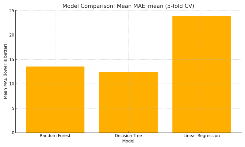
Figure 3: Model comparison based on Mean MSE (5‑fold CV). Random Forest achieved the lowest MSE.

Figure 4: Predicted vs Actual salaries using Random Forest on the hold‑out test set. Points near the 45° line indicate accurate predictions.

Figure 5: Top 10 features influencing salary prediction according to the Random Forest model.

• Results Interpretation 

• The Random Forest Regressor was the most successful model, as evidenced by its highest R2 and lowest error. As expected with real-world pay data, minor deviations from the regression line show some variation brought on by outliers.

Social Impact

The Salary Prediction System can help professionals figure out what they might earn depending on the state they choose to work in. Based on the input fields customers have filled out, the model is able to provide the projected salary. Professionals can assess their own worth in the state or sector they want to work in by knowing how much they would be paid based on state, sector, job role, job tenure, etc.

Knowing this information can assist professionals choose the state where they want to work. In accordance with your desired employment role and seniority, they can also see what you will be paid. People can use this initiative to help them plan their future.

Limitations

In this case, if the user wishes to determine salary based on work experience, skills, etc., the entire procedure is carried out with state-based compensation prediction in mind. Due to the fact that this model’s goal is distinct from that, it cannot be used for that purpose. Additionally, we can see that the acquired data has limitations due to its limited number of 956 rows.

Conclusion

Using machine learning techniques, this research successfully created a pay prediction model for data-related roles in the US.  Important results include: 

• Compared to Linear Regression and Decision Tree Regressor, Random Forest Regressor had the highest accuracy (R2 = 0.9678). 

• The predictive power of the model was greatly enhanced by feature engineering, which included extracting talents (Python, AWS, Spark) and firm attributes (size, revenue, age). 

• It was discovered that seniority and geographic location were significant predictors of compensation differences. 

• The model can aid businesses in creating competitive compensation packages and job seekers in estimating expected salaries. 

References

Skit Learn. (2023, April 7). Linear Regression. Skit Learn. https://scikit-learn.org/stable/modules/generated/sklearn.linear_model.LinearRegression.html

Real Python. (2023, February 7). Pythonic data cleaning with pandas and NumPy. Real Python. https://realpython.com/python-data-cleaning-numpy-pandas/

Pickle – python object serialization. Python documentation. (n.d.). https://docs.python.org/3/library/pickle.html

Streamlit docs. Streamlit documentation. (n.d.). https://docs.streamlit.io/

D’Agostino, A. (2023, April 4). Exploratory Data Analysis in python - a step-by-step process. Medium. https://towardsdatascience.com/exploratory-data-analysis-in-python-a-step-by-step-process-d0dfa6bf94ee

Sklearn.model_selection.train_test_split. scikit. (n.d.). https://scikit-learn.org/stable/modules/generated/sklearn.model_selection.train_test_split.html

Sklearn.model_selection.GRIDSEARCHCV. scikit. (n.d.-c). https://scikit-learn.org/stable/modules/generated/sklearn.model_selection.GridSearchCV.html

Menon, K. (2023, March 10). Types of machine learning: Simplilearn. Simplilearn.com. https://www.simplilearn.com/tutorials/machine-learning-tutorial/types-of-machine-learning

Sklearn.linear_model.linearregression. scikit. (n.d.-a). https://scikit-learn.org/stable/modules/generated/sklearn.linear_model.LinearRegression.html

Statsmodels.regression.linear_model.ols. statsmodels.regression.linear_model.OLS – statsmodels 0.15.0 (+6). (n.d.). https://www.statsmodels.org/devel/generated/statsmodels.regression.linear_model.OLS.html

Sklearn.tree.decisiontreeregressor. scikit. (n.d.-c). https://scikit-learn.org/stable/modules/generated/sklearn.tree.DecisionTreeRegressor.html

Sklearn.ensemble.randomforestregressor. scikit. (n.d.-a). https://scikit-learn.org/stable/modules/generated/sklearn.ensemble.RandomForestRegressor.html

Pant, A. (2019, January 23). Workflow of a machine learning project. Medium. https://towardsdatascience.com/workflow-of-a-machine-learning-project-ec1dba419b94