Thesis : Nepali Text Document Classification using Deep Neural Networks

Declaration of the Student

I hereby certify that I am the sole author of this work and that it has solely used the sources that are specified above.

……………..

Roshan Sah

Suggestion from the Supervisor

I hereby suggest that this dissertation, ” An In-Depth Proposal for Nepali Text Document Classification Leveraging Deep Neural Networks” completed under the guidance of Dr. Sushil Shrestha, be processed for evaluation in partial fulfilment of the requirements for the degree of MSC IT IN DATA ANALYTICS.

.. ……………

Dr. Sushil Shrestha

PhD in Learning Analytics

Assistant Professor | Department of Computer Science and Engineering (DoCSE)

Kathmandu, Nepal

Date: May, 2024

APPROVAL LETTER

We attest that we have read this dissertation and that, in our judgement, it satisfies the requirements for both scope and quality as a dissertation for the master’s degree in computer science and information technology.

Evaluation Committee

……………………………….Dr. Sushil ShresthaPhD in Learning AnalyticsAssistant Professor | Department of Computer Science and Engineering (DoCSE)Kathmandu, Nepal (Head)

………………………………Dr. Sushil ShresthaPhD in Learning AnalyticsAssistant Professor | Department of Computer Science and Engineering (DoCSE)Kathmandu, Nepal (Supervisor)

……………………
(Internal examiner)

……………………(External examiner)

Date: May, 2024

ACKNOWLEDGEMENTS

Above all, I am immensely grateful to my supervisor, Dr. Sushil Shrestha. This job would have been difficult to achieve without their assistance, involvement, encouragement, and support. I greatly appreciate your extensive support and profound understanding.

I would like to convey my profound appreciation to Islington College for granting me a scholarship that greatly facilitated the smooth execution of my research project.

I would like to convey my appreciation to all those who provided support to me during the duration of my research work for my M.Sc. IT.

I express my sincere gratitude to all the faculty members and staff of Information Technology for their generous assistance and cooperation during my academic tenure.

I would want to extend my appreciation to all individuals who have been directly or indirectly involved in assisting me in completing my research project.

Lastly, I would want to express my gratitude to my family and friends for their unwavering support and encouragement during my research endeavor.

Roshan Sah

May, 2024

ABSTRACT

The objective of a document categorization task is to allocate a document to one or many classes or categories. This research examines the categorization of Nepali and English text documents using neural networks such as RNN (Recurrent Neural Network) and MNN (Multi Neural Network). It also compares the performance of RNN and MNN based on established performance assessment parameters. The experimental findings demonstrated that the Recurrent Neural Network (RNN) had superior performance compared to the Multilayer Neural Network (MNN).

Keywords: Document classification, Recurrent Neural Network (RNN), Multilayer Neural Network (MNN), Neural Network, Artificial Intelligence (AI)

Table of Contents

CHAPTER 1

INTRODUCTION

1.1 Overview

1.1.1 An artificial neural network

1.1.2 RNN (Recurrent Neural Network)

1.2 Problem Statement

1.3 Objectives

1.4 Structure of the report

CHAPTER 2

BACKGROUND AND LITERATURE REVIEW

2.1 Background

2.1.1 Neural Network Model

2.1.2 Multiple Neural Network

2.1.3 Activation Function

2.1.4 SoftMax Function

2.1.5 Cross-Entropy Loss Function

2.1.6 Gradient Descent Algorithm

2.1.7 A Deep Network Problem with Vanishing/Explosing Gradient

2.1.8 Propagation backward

2.1.9 LSTM (Long Short-Term Memory)

2.2 Literature Review

CHAPTER 3

RESEARCH METHODOLOGY

3.1 Data Set Preparation

3.1.1 Preprocessing

3.1.2 Data Vectorization

3.2 Steps in Text classification

3.3 Performance Evaluation Parameter

4.1 Multi-Neural Network

4.2 Recurrent Neural Network

4.3 Mathematical Implementation of Classifier

4.4 Programming Language and TensorFlow

CHAPTER 5

RESULT AND ANALYSIS

5.1 Experimental Setup

5.1.1 Data set

5.1.2 Splitting the dataset into training and testing sets

5.1.2.1 Conducting the Experiment 1

5.1.2.2 Conducting the Experiment 2

5.1.2.3 Conducting the Experiment 3

5.1.2.4 Conducting the Experiment 4

5.1.2.5 Conducting the Experiment 5

5.1.2.6 Conducting the Experiment 6

5.1.2.7 Conducting the Experiment 7

5.1.2.8 Conducting the Experiment 8

5.1.2.9 Conducting the Experiment 9

5.1.2.10 Conducting the Experiment 10

5.2 Bar Chart Analysis of Result of Experiment

5.2.1 Nepali Dataset test with 20% of sample data for MNN with all 5 experiments

5.2.2 Nepali Dataset test with 20% of sample data for RNN

CHAPTER 6

DISCUSSION

6.1 Summary of Results

6.2 Practical/Theoretical/Managerial/Research Contribution

6.3 Limitations

6.4 Benefits

CHAPTER 7

CONCLUSION AND RECOMMENDATION

LIST OF TABLES

Table 1Vector representation of sentences

Table 2 Confusion Matrix for the sample

Table 3 No of sample on Train set

Table 4 No of sample on Test set for specific class

Table 5 Hyperparameters and final loss

Table 6 Confusion matrix for Nepali Data of MNN

Table 7 Hyperparameters and final loss

Table 8 Confusion matrix for Nepali Data of MNN

Table 9 Hyperparameters and final loss

Table 10 Confusion matrix for Nepali Data of MNN

Table 11 Hyperparameters and final loss

Table 12 Confusion matrix for Nepali Data of MNN

Table 13 Hyperparameters and final loss

Table 14 Confusion matrix for Nepali Data of MNN

Table 15 Hyperparameters and final loss

Table 16 Confusion matrix for Nepali Data of MNN

Table 17 Hyperparameters and final loss

Table 18 Confusion matrix for Nepali Data of MNN

Table 19 Hyperparameters and final loss

Table 20 Confusion matrix for Nepali Data of MNN

Table 21 Hyperparameters and final loss

Table 22 Confusion matrix for Nepali Data of MNN

Table 23 Hyperparameters and final loss

Table 24 Confusion matrix for Nepali Data of MNN

TABLE OF FIGURES

Figure 1 working of single-layer perceptron network

Figure 2 Graph of ReLU mapping input to corresponding output.

Figure 3 Graph of Tanh activation function mapping input to corresponding output.

Figure 4 gradient descent when slope is positive.

Figure 5 gradient descent when slope is negative

Figure 6 Simple Recurrent Neural Network (RNN) with BPTT

Figure 7 block diagram of RNN cell.

Figure 8 block diagram of LSTM cell.

Figure 9 Block Diagram of Steps in Text Classification

Figure 10 Block Diagram of Over All Classification System

Figure 11 Simple multi-layer neural network

Figure 12 Simple Recurrent Neural Network (RNN)

Figure 13 Block diagram of Data flow graph of TensorFlow

Figure 14 Bar chart for Nepali Data of MNN

Figure 15 Bar chart for Nepali Data of RNN

Figure 16 dataset sample from business category

Figure 17 dataset sample from interview category

Figure 18 preparation of dataset from text

Figure 19 python script to filter data set

Figure 20 python script to shape data set

Figure 21 python script to train model

Figure 22 gaant chart defining time spent in each step of the project

Figure 23 originality report 1

Figure 24 originality report 2

CHAPTER 1 INTRODUCTION

1.1 Overview

Deep Learning is a recently developed field of research within Machine Learning that aims to bring Machine Learning closer to its original purpose of achieving Artificial Intelligence.

Artificial intelligence (AI), sometimes known as machine intelligence (MI), refers to the intelligence exhibited by machines, as opposed to the natural intelligence (NI) observed in humans and other animals. AI research in computer science is the investigation of “intelligent agents,” which refers to any technology capable of seeing its surroundings and making decisions that optimize its likelihood of accomplishing its objectives [P. David, 1998]. Artificial intelligence refers to the application of machines that imitate “cognitive” functions associated with human minds, such as “learning” and “problem solving” [G. Brewka, 2009]. Artificial intelligence (AI) is a field within computer science that focuses on developing machines capable of performing tasks and responding in a manner similar to humans. Artificial intelligence is a discipline within computer science that seeks to develop machines capable of exhibiting intelligent behavior. It has become a crucial component of the technological sector.

Machine learning is a branch of computer science that employs statistical methods to enable computer systems to learn and enhance their performance on a particular task using data, without the need for explicit programming [A. L. Samuel, 1969]. Machine learning and computational statistics are intimately intertwined, having significant overlap in their objectives of utilizing computers to make predictions. The field has a close relationship with mathematical optimization, which provides methods, theory, and application domains. Machine learning is occasionally confused with data mining.

Deep learning is a subset of machine learning techniques that focus on learning data representations rather than using unique algorithms for each task. Learning can be categorized into three types: supervised, semi-supervised, or unsupervised [J. Schmindhuber, 2015]. Deep learning models have been utilized in various domains such as computer vision, speech recognition, natural language processing, audio recognition, and social network filtering. In these areas, these models have achieved outcomes that are equivalent to, and in certain instances, surpass human expertise [D. Ciregan, 2012].

Deep learning refers to a category of machine learning algorithms that are characterized by their depth and complexity.

❖ Employ a series of interconnected layers of nonlinear processing units to extract and transform features. Each subsequent layer use the output from the preceding layer as its input.

❖ Learning can be either supervised, such as in classification tasks, or unsupervised, such as in pattern analysis.

❖ Acquire knowledge about many layers of representations that correspond to different degrees of abstraction; these layers create a hierarchical structure of concepts.

This study examines the efficacy of Recurrent Neural Networks (RNNs) and Multi Neural Networks (MNNs) in classifying Nepali text documents. The primary objective is to analyse how different hyperparameter configurations affect their performance. The objective of the study is to assess and contrast the effectiveness and precision of Recurrent Neural Networks (RNNs) and Multilayer Neural Networks (MNNs) in the task of categorising documents. Additionally, the study intends to pinpoint the main obstacles encountered while employing these advanced learning algorithms on Nepali language. In addition, the project aims to identify techniques for enhancing the efficiency of Recurrent Neural Networks (RNNs) and Multilayer Neural Networks (MNNs) in this specific scenario. Furthermore, this study also investigates the practical consequences of employing these algorithms for real-life applications in the classification of Nepali text documents. The classification method pays particular attention to how RNNs and MNNs deal with the intricacies of the Nepali language, including morphology, syntax, and semantics.

1.1.1 An artificial neural network

An artificial neural network (ANN) or neural network is a type of computing system that is designed based on the structure and function of biological neural networks found in brains. These systems enhance their performance on tasks by learning from examples, typically without the need for programming specialised to the task. Artificial intelligence (AI) has made significant progress, enabling the use of artificial neural networks (ANNs). Artificial Neural Networks (ANNs) are capable of efficiently solving intricate issues within a realistic timeframe. Artificial Neural Networks (ANNs) are conceptual tools that facilitate the comprehension of how neural input is processed [M. van Gerven, 2017].

An artificial neural network (ANN) is constructed from interconnected units or nodes known as artificial neurons. Every link between artificial neurons has the ability to convey a signal from one neuron to another. The artificial neuron that receives the signal has the ability to analyze and interpret it, and subsequently transmit signals to other artificial neurons that are linked to it.

1.1.1.1 The mathematical representation of an artificial neuron

In figure 1, the functioning of multi-neural networks can be comprehended by examining the operations of a single layer neural network. In a multi-neural network, the computing method remains unchanged, but more hidden layers are incorporated into the network.

Figure 1 working of single-layer perceptron network

1.1.2 RNN (Recurrent Neural Network)

A recurrent neural network (RNN) is a type of artificial neural network in which the units are connected in a directed graph along a sequence. This enables it to demonstrate dynamic temporal behaviour during a sequence of time. Recurrent Neural Networks (RNNs) have the ability to utilise their internal state, or memory, to handle sequences of inputs. Recurrent neural networks (RNNs) possess cyclic connections, which enhance their capability to effectively describe sequential input. [H. Sak, 2018]

In a conventional neural network, it is assumed that all inputs are independent of one another. However, recurrent neural networks (RNNs) incorporate the concept of input dependencies within words. For example. In order to anticipate the following word in a sentence, Recurrent Neural Networks (RNNs) retain information about words that have been seen a few steps earlier. RNNs are referred to as recurrent because they execute the same operation for each element in a sequence, and the outcome is dependent on the prior calculations. While theoretically, Recurrent Neural Networks (RNNs) have the capability to utilise information from sequences of any length, in practice, they are constrained to only consider a small number of preceding steps. The Recurrent Neural Network employs the backpropagation algorithm, which is utilised for every time step. Backpropagation Through Time (BTT) is a well-recognised term for this concept.

1.2 Problem Statement

Optimally, within the realm of text analysis, the classifier should accurately assign incoming documents to the appropriate pre-established categories used during training, while also identifying documents that do not fit into any of the established categories. This issue is referred to as open world classification or open classification. [G. Fei, 2015]

A vast amount of unstructured and disorganised data is readily available in the digital realm. Directly utilising the data from the source is impracticable due to its unstructured nature. In order to derive any benefit from the supplied data, it is necessary to organise the textual data.

The MNN and RNN approaches are utilised for document classification. This research aims to investigate the impact of varying hyperparameter settings on the performance of a neural network model and to determine the efficiency of MNN and RNN for document categorization.

The task of analysing and categorising text documents is especially challenging when it comes to the Nepali language. This is because Nepali has distinct linguistic features and there is a large amount of unstructured and disorganised textual data available in digital form. The absence of a well-defined organisational structure in this data frequently hinders the direct extraction of significant insights from the source. Conventional methods for document categorization face difficulties in handling the intricacies of natural language, including the subtleties of syntax, context, and semantics, which are particularly prominent in Nepali literature. In addition, the current body of research on deep learning methods, such as Multi Neural Networks (MNNs) and Recurrent Neural Networks (RNNs), mainly concentrates on languages with extensive collections of texts and well-established datasets. Consequently, there is a lack of application of these techniques to less researched languages like Nepali. This study seeks to close this disparity by examining the efficacy of MNNs and RNNs in classifying Nepali text texts. This study aims to gain useful insights into the application of sophisticated machine learning techniques in efficiently organising and categorising unstructured Nepali text data by examining the effects of various hyperparameter settings on the efficiency and accuracy of deep learning models.

1.3 Objectives

The primary goals of this research are to categorise textual data in the form of text documents using deep learning algorithms such as Recurrent Neural Network (RNN) and Multi Neural Network (MNN). Deep learning computational approaches are utilised to uncover valuable information that is concealed inside data and subsequently categorise it.

1.4 Structure of the report

Chapter 1 introduces deep learning and artificial neural networks, emphasizing their role in advancing machine learning towards artificial intelligence. Chapter 2 covers neural network models, activation functions, and gradient descent algorithms, along with a literature review. Chapter 3 explains dataset preparation, text classification steps, and performance evaluation. Chapter 4 details the implementation of Multi-Neural Network and Recurrent Neural Network models, including mathematical implementations and the use of TensorFlow. Chapter 5 presents the experimental setup and analysis, including ten experiments and results using bar charts. Chapter 6 summarizes the findings and provides recommendations for future research.

CHAPTER 2 BACKGROUND AND LITERATURE REVIEW

2.1 Background

2.1.1 Neural Network Model

2.1.2 Multiple Neural Network

The Multi-layer neural network, also known as the multi-layer perceptron (MLP), is composed of three or more layers. These levels include an input layer, an output layer, and one or more hidden layers. The nodes within these layers are activated in a nonlinear manner, which gives the network its deep structure. The multilayer perceptron is widely recognised as the most prominent and commonly employed form of neural network. Typically, the signals inside the network are transferred unidirectionally, moving from the input to the output. There is no feedback loop in which the output of a neuron influences its own activity. The term used to describe this architecture is “feedforward”. Additionally, there exist feedback networks that have the ability to transmit impulses in both directions as a result of the presence of response links inside the network. These networks possess significant computational capabilities and can be highly intricate [M. Popescu, 2009].

MLPs, or Multi-Layer Perceptron’s, are characterised by their fully linked structure, where each node in one layer is coupled to every node in the subsequent levels through weighted connections. The backpropagation technique is employed to modify the weights in the network. The activation function of a node determines the resulting output of that node.

2.1.3 Activation Function

In computational networks, the activation function of a node determines the output of that node based on a particular input or combination of inputs. A typical computer chip circuit can be viewed as a digital network consisting of activation functions that can be in either a “ON” state (1) or a “OFF” state (0), depending on the input. The activation function plays a crucial role in mapping specific outputs to specific sets of inputs.

2.1.3.1 Rectified Linear Unit (ReLU) Activation Function

The Rectified Linear Unit (ReLU) activation function is utilised in the implementation of the Multi-Neural Network [G. E. Hinton, 2003]. The ReLU function has a domain of all real numbers and a range of values between 0 and 1. The equation representing the boundary of the Rectified Linear Unit (ReLU) is displayed below.

Figure 2 Graph of ReLU mapping input to corresponding output.

Figure 2 depicts the process of assigning input values to their corresponding output values using the Rectified Linear Unit (ReLU) activation function. It showcases the distinct linear segments of the function that intersect at the origin.
2.1.3.2 Tanh activation function

Tanh activation function is implemented for the Recurrent Neural Network.

The range of the tanh function is from -1 to 1

Figure 3 illustrates the Tanh activation function, showcasing how it maps input values to corresponding output values within the range of -1 to 1.

Figure 3 Graph of Tanh activation function mapping input to corresponding output.

2.1.4 SoftMax Function

The SoftMax function takes the output of a neural network, such as o₁ from the figure above, as input and produces the output as a probability distribution.

The SoftMax function ensures that the outputs of the neural network add up to 1, allowing them to reflect a probability distribution across mutually incompatible discrete outputs.

The SoftMax function is defined as follows : [Z. Zhang, 2018]

2.1.5 Cross-Entropy Loss Function

The cost function utilised during the training of the neural network model is cross-entropy. The cross-entropy loss function is a technique used to quantify the difference between the projected probability of a neural network model and the expected label or class [Z. Zhang, 2018].

Cost function is given by,

The value of L (loss function) is regarded low when there is a small difference between the predicted probability of the neural network model and the expected result. This indicates that the error or loss of the neural network model is low. Conversely, if the value of L (loss function) increases, it means that there is a larger difference between the projected probability and the expected result.

2.1.6 Gradient Descent Algorithm

Gradient descent is an iterative optimisation process used to discover the minimal value of a function. It operates by taking steps in the direction of the negative gradient of the function. In order to locate a local minimum of a function using gradient descent, one must take steps that are proportional to the negative of the gradient (or an approximation of the gradient) of the function at the current position. If one takes steps proportional to the negative of the gradient, one will move towards a local maximum of the function. This process is referred to as gradient descent.

Figure 4 gradient descent when slope is positive.

2.1.7 A Deep Network Problem with Vanishing/Explosing Gradient

During the training of a neural network model, the issue of vanishing or exploding gradient arises when the derivative of the cost function becomes either exponentially large or exponentially tiny. This phenomenon hinders the training process and makes it challenging.

The Vanishing/Exploding Gradient problem occurs while training a neural network model with backpropagation, particularly in the case of RNNs. During the occurrence of the problem, the duration of the training process is too lengthy, resulting in a decline in accuracy.

During the training process, the neural network continuously computes the cost value. The cost value is calculated as the discrepancy between the anticipated output value of a neural network and the expected value derived from a set of labelled training data.

Cost is minimized by iteratively adjusting the weights during the training phase until the cost value reaches its minimum.

The training method employed a gradient, which quantifies the speed at which the cost will vary in response to a modification in a weight.

2.1.7.1 The disappearing gradient

Neural networks train at a slower pace when the gradient is extremely tiny. The gradient may potentially diminish or dissipate as it propagates through the neural network, causing the initial layers of the network to have the slowest training speed.

The vanishing gradient problem results in the network primarily retaining information from recent occurrences while disregarding information from more distant earlier events. The gradient at any given position is the cumulative result of multiplying the gradients from all preceding points leading up to that point.

2.1.7.1 The Exploding gradient

The phenomenon known as “exploding gradient” refers to the issue of gradients in a neural network becoming extremely large during the training process.

Neural networks train rapidly when the gradient is significantly large. Exploding gradients refer to the issue of significant error gradients accumulating and leading to substantial modifications in the weights of a neural network model during the training process. This leads to instability and an inability of the neural network model to learn from the training data.

2.1.8 Propagation backward

During the training of the network, the loss function (cross-entropy) quantifies the error of the neural network model. The error or cost of the neural network model is determined by calculating the difference between the anticipated output value and the expected output value [D. E. Rumelhart, 1985]. A neural network model computes the error in order to backtrack through the network and modify the weights, aiming to minimize the error in subsequent iterations. Gradient descent is employed to minimize the error of the neural network model. The backpropagation algorithm iteratively adjusts the weights of the neural network by propagating information backwards through the network. This procedure is done for each input in the training dataset. This process is iterated until the error diminishes to a magnitude that allows it to be considered as trained.

2.1.8.1 Back Propagation Through Time (BPTT)

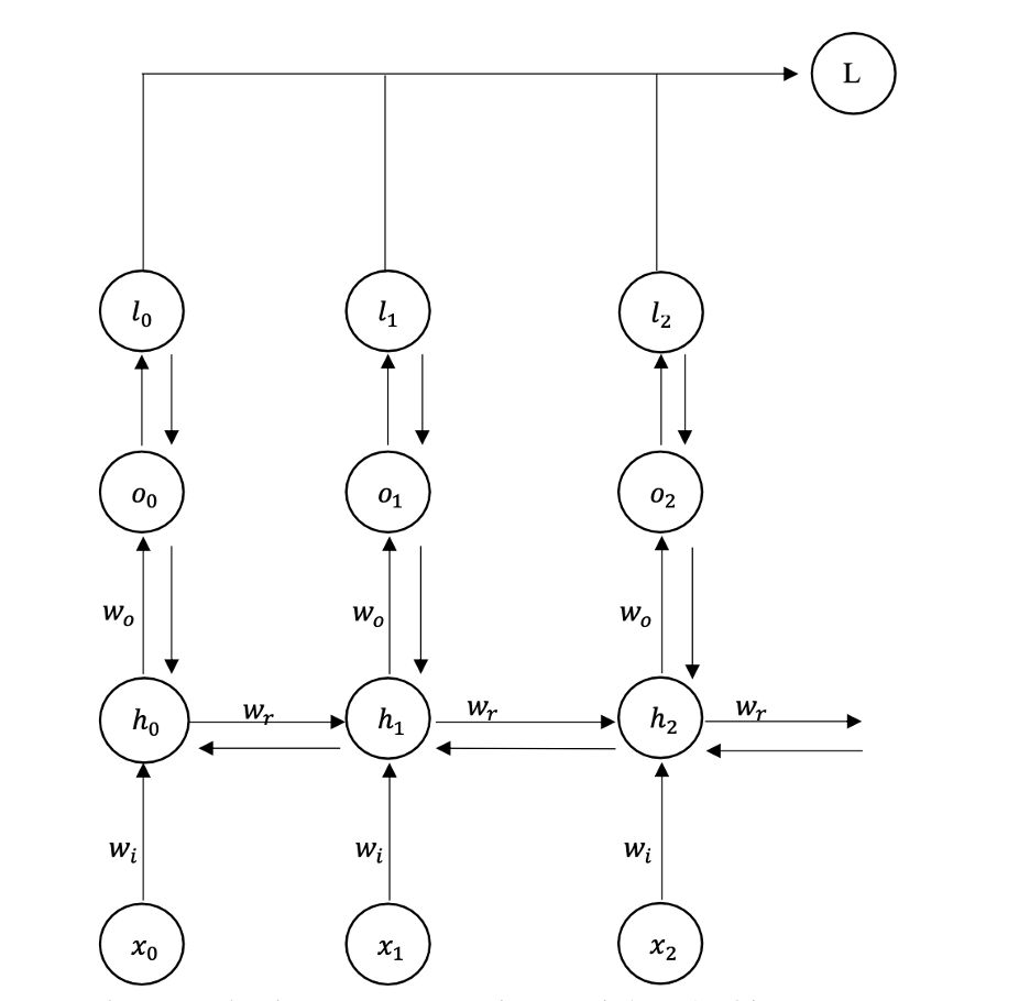
Figure 6 Simple Recurrent Neural Network (RNN) with BPTT

Figure 6 illustrates a Simple Recurrent Neural Network (RNN) with Back Propagation Through Time (BPTT). This process involves computing the error starting from the final output and propagating it backward through the network to adjust the weights and minimize the error.

Backpropagation in feedforward networks involves the reverse movement of information, starting at the final mistake and going through the outputs, weights, and inputs of each hidden layer. The error is computed and an optimizer is subsequently employed to modify the weight, resulting in a reduction of the error.

The loss function is necessary for calculating the backpropagation.

Backpropagation performs computations in the opposite direction of all the steps involved in forward propagation. The backpropagation procedure enables the computation of suitable quantities and the updating of the parameters of the neural network model in order to minimise the generated error.

BPTT use gradient descent to update the weights and biases of a neural network, therefore minimising the error in the network.

2.1.9 LSTM (Long Short-Term Memory)

Long short-term memory (LSTM) units, also known as blocks, serve as fundamental components for the layers of a recurrent neural network (RNN). An RNN consisting of LSTM units is sometimes referred to as an LSTM network. A typical LSTM unit consists of a cell, an input gate, an output gate, and a forget gate. The primary function of the cell in LSTM is to retain and recall information for extended periods, which is why it is referred to as “memory”. Each of the three gates can be conceptualised as a “conventional” artificial neuron, similar to those found in a multi-layer (or feedforward) neural network. In other words, they calculate an activation value by applying an activation function to a weighted sum. Conceptually, they can be understood as controllers of the movement of values that traverse the connections of the LSTM [H. Sak, 2018].

The RNN cell is a basic component that calculates the inputs and bias.

Figure 7 block diagram of RNN cell.

2.2 Literature Review

Warren McCulloch and Walter Pitts developed a computational model for neural networks known as threshold logic in 1943. This model was based on mathematical principles and algorithms. This model was helpful in advancing neural network research. The paper elucidated the functioning of neurons. To elucidate the functioning of neurons in the brain, they constructed a rudimentary neural network by employing electrical circuits [W. S. Mcculloch, 1990]. In 1949, Donald Hebb authored The Organisation of Behaviour, which highlighted the crucial fact that brain pathways are reinforced with each use, a concept that is critically vital to human learning processes. According to his argument, if two nerves simultaneously generate electrical impulses, the strength of the link between them is increased.Rosenblatt (1958) developed the perceptron, an algorithm designed for the purpose of pattern recognition. Rosenblatt utilised mathematical notation to explain circuitry that went beyond the fundamental perceptron, including the exclusive-or circuit, which was not capable of being processed by neural networks during that period [P. J. Werbos, 1974]. This played a crucial role in the subsequent development of the neural network. In 1962, Widrow and Hoff devised a learning algorithm that evaluates the value prior to adjusting the weight (either 0 or 1) based on the following rule:

Weight Change = (Value before weight adjustment) * (Error / (Number of Inputs)).

The concept behind this approach is that if a single active perceptron has a significant error, the weight values can be adjusted to disseminate the error throughout the network, or at least to neighbouring perceptrons. Even when this rule is applied, an error still occurs if the line preceding the weight is 0. However, this problem will eventually be resolved on its own. If the error is evenly spread among all the weights, it will be completely eradicated. They devised a learning algorithm that evaluates the value prior to adjusting the weight. Neural network research saw a lack of progress following the machine learning research conducted by Minsky and Papert in 1969. They identified two fundamental problems with the computational devices used to analyse neural networks. One limitation of basic perceptrons was their inability to comprehend the exclusive-or circuit. The second issue was the insufficient computational capacity of computers to efficiently manage the computational demands of huge neural networks. Progress in neural network research was hindered until computers attained significantly enhanced processing capabilities. In 1975, the first unsupervised multilayered network was established. Rina Dechter proposed the term Deep Learning to the machine learning field in 1986, while Igor Aizenberg and colleagues launched Artificial Neural Networks in 2000. In 1998, Support Vector Machines were utilised for text classification [T. Joachims, 2018]. In 2000, Schapire and Singer improved AdaBoost to effectively handle multiple labels. The approach demonstrated involves treating the task of assigning many subjects to a text as a process of ranking labels for the text. The motivation for this evaluation was derived from the field of Information Retrieval. In 2009, the notion of neural networks resurfaced under a new name, deep learning, introduced by Hinton. In their 2018 study titled “Weakly-Supervised Neural Text Classification,” Yu Meng, Jiaming Shen, Chao Zhang, and Jiawei Han conducted a comparative analysis of the classification capabilities of various neural classifiers. The experiment involved assessing the practical effectiveness of their approach for text classification under weak supervision. The authors suggested a text categorization approach that relies on neural classifiers and is based on weak supervision. This study was notable since it demonstrated that the approach performed better than the baseline methods to a large degree. Additionally, it showed that the method was highly resilient to variations in hyperparameters and different types of user-provided seed information. The suggestion was made to research the effective integration of various types of seed information in order to enhance the performance of the method. The number 19 is enclosed in square brackets. In their 2018 work titled “Practical Text Classification With Large Pre-Trained Language Models,” Neel Kant, Raul Puri, Nikolai Yakovenko, and Bryan Catanzaro discussed the application of large pre-trained language models.The researchers conducted a comparison between the deep learning architectures of the Transformer and mLSTM and discovered that the Transformer outperforms the mLSTM in all categories.The researchers showcased that employing unsupervised pretraining and finetuning offers a versatile framework that proves to be very efficient for challenging text categorization tasks. The researchers discovered that the process of fine-tuning yielded particularly favourable results when applied to the transformer network [N. Kant, R. Puri, 2020]. In their study titled “Long Short-Term Memory Recurrent Neural Network Architectures for Large Scale Acoustic Modelling,” Has ̧Im Sak, Andrew Senior, and Franc ̧Oise Beaufays assessed and compared the effectiveness of LSTM RNN designs in the context of a high-volume voice recognition task known as the Google Voice Search task. The acoustic modelling in this study employed a hybrid technique, combining LSTM RNNs with neural networks to estimate the hidden Markov model (HMM) state posteriors. The researchers demonstrated that deep LSTM RNN architectures reach the highest level of performance for large-scale acoustic modelling. The suggested deep LSTMP RNN structure surpasses the performance of conventional LSTM networks [H. Sak, 2018].

In 1986, Rina Dechter made a significant breakthrough in the field of machine learning by coining the phrase “Deep Learning.” This introduction represented a noteworthy achievement in the advancement of artificial neural networks and the wider field of artificial intelligence. Dechter’s research established the basis for a new era of investigation and practical uses, significantly altering the way neural networks are understood and employed. Prior to Dechter’s invention of deep learning, neural networks were predominantly shallow, comprising only a limited number of layers. Although these networks have their utility in specific tasks, they have inherent limitations when it comes to representing intricate patterns and relationships in data. Deep learning popularised the notion of deep neural networks, which are distinguished by their numerous layers of interconnected neurons. The utilisation of deep architectures allows the networks to acquire hierarchical representations of data, collecting increasingly abstract and complex aspects at higher layers. Dechter’s notion of deep learning highlighted the significance of incorporating multiple layers in neural network topologies. Deep learning models can enhance their ability to extract complex features and recognise patterns by adding more layers. The depth of the models enables them to enhance and expand upon the basic characteristics recognised in previous layers, hence allowing them to identify and comprehend more intricate structures. The power and versatility of deep learning stem from its hierarchical learning process, which allows it to surpass typical shallow networks in a diverse array of tasks. Dechter’s introduction of deep learning has a significant impact that goes beyond theoretical achievements. This resulted in a surge of research and development that resulted in notable practical advancements in diverse fields, such as computer vision, natural language processing, speech recognition, and game playing. The efficacy of deep learning models in various domains has showcased their capacity to effectively extrapolate from extensive datasets, becoming them indispensable for both scholarly investigations and industry implementations. One significant advancement that occurred after Dechter’s presentation was the enhancement of training algorithms for deep networks. Methods such as backpropagation and stochastic gradient descent were improved to effectively deal with the heightened intricacy of deep structures. Furthermore, the progress in processing capacity and the accessibility of extensive datasets facilitated the feasible training of deep learning models, which were previously computationally unaffordable. Dechter’s contribution emphasised the necessity of employing efficient regularisation approaches to mitigate overfitting in deep networks. Techniques such as dropout, batch normalisation, and data augmentation were created to tackle this difficulty, hence improving the effectiveness and resilience of deep learning models. These advancements have played a vital role in guaranteeing that deep learning models exhibit strong generalisation capabilities when presented with unfamiliar data, thereby establishing their reliability for practical use. Ultimately, the introduction of the phrase “Deep Learning” by Rina Dechter in 1986 had a profound impact on the development of artificial intelligence and machine learning. It introduced a novel framework for studying neural networks, highlighting the significance of incorporating several layers in brain structures. Dechter’s research established the foundation for later progress that has resulted in the extensive acceptance and achievement of deep learning models in several domains. Her contribution has a lasting impact on the trajectory of AI research and the advancement of cutting-edge products that leverage the potential of deep learning [Dechter, 1986].

In 2000, Igor Aizenberg and his colleagues made notable advancements in the field of artificial neural networks (ANNs) with their groundbreaking research. Aizenberg et al. largely concentrated on improving the computing capabilities and practical uses of neural networks, which have subsequently become fundamental in the wider field of machine learning and artificial intelligence. Aizenberg et al. played a crucial role in the advancement and use of Multi-Valued and Complex-Valued Neural Networks (MVNNs and CVNNs). These neural networks expanded the conventional binary and real-valued models to include multi-valued and complex domains, allowing for more advanced data representations and processing capabilities. The implementation of these networks resolved certain constraints of traditional ANNs, including in managing intricate input patterns and executing resilient function approximations. Aizenberg and his team’s research emphasised the theoretical and practical advantages of MVNNs and CVNNs. These networks have been demonstrated to provide enhanced learning efficiency and generalisation capabilities, rendering them appropriate for many applications like as image and signal processing, pattern recognition, and data compression. By integrating complicated numbers into the neural network architecture, researchers achieved the ability to simulate and analyse data in ways that were previously unachievable using conventional artificial neural networks. An important achievement of this research was the creation of algorithms that made it easier to train and optimise MVNNs and CVNNs. The algorithms developed by Aizenberg et al. were specifically intended to take use of the distinct characteristics of multi-valued and complex-valued representations. This design choice aims to improve the speed at which the learning process converges and enhance its stability. These developments not only enhanced the efficiency of neural networks in existing tasks but also broadened their suitability for novel and more demanding issues. Aizenberg et al. investigated the incorporation of MVNNs and CVNNs with various neural network topologies and learning methodologies. This interdisciplinary approach facilitated the construction of hybrid models that integrated the advantages of many neural network topologies, resulting in computational systems that are more adaptable and robust. The integration efforts showcased the capacity of these sophisticated neural networks to surpass standard models in multiple domains. Overall, the work of Igor Aizenberg and his colleagues in 2000 represented a noteworthy advancement in the development of artificial neural networks. Their study on Multi-Valued and Complex-Valued Neural Networks expanded the scope of the science, enhancing the efficacy and efficiency of data processing. Aizenberg et al.’s theoretical discoveries and practical implementations have significantly influenced the development of neural network technology, shaping subsequent research and applications in machine learning and artificial intelligence [Aizenberg, 2000].

Practical Text Classification With Large Pre-Trained Language Models authored by Neel Kant, Raul Puri, Nikolai Yakovenko, and Bryan Catanzaro investigates the use of extensive pre-trained language models for tasks involving text classification. This topic holds great importance within the field of natural language processing (NLP), where the precise classification and comprehension of text are vital for a range of applications, such as information retrieval, sentiment analysis, and content suggestion. The researchers conducted a comparative analysis of the performance of two deep learning architectures: the Transformer and the multi-layer Long Short-Term Memory (mLSTM). The Transformer architecture, renowned for its self-attention mechanism, enables the model to assess the significance of various words in a phrase, hence enhancing its ability to capture long-range dependencies more efficiently compared to conventional RNNs. On the other hand, mLSTM networks employ a sequence of LSTM layers to handle sequential data, ensuring that context is preserved across larger sequences. The authors’ research revealed the superior performance of the Transformer design compared to the mLSTM in a range of text categorization tasks. The Transformer’s exceptional performance can be attributed to its capability to effectively handle long-range relationships and its efficient utilisation of computational resources. The study also emphasises the efficacy of unsupervised pre-training followed by fine-tuning for targeted activities. This method utilises extensive quantities of unlabeled text data to acquire comprehensive language representations, which are subsequently adjusted for specific classification tasks using supervised learning. The study emphasises the tangible advantages of employing extensive pre-trained language models in realistic scenarios. The method of fine-tuning has been demonstrated to produce outstanding outcomes by improving the model’s performance on certain tasks, with the need for only a moderate amount of labelled data related to the task. This technique is extremely scalable and cost-effective for a wide range of natural language processing (NLP) applications. Moreover, the work offers valuable understanding regarding the strength and adaptability of extensive pre-trained models. The authors noted that these models demonstrate robustness to changes in hyperparameters and are capable of efficiently using diverse input data. The robustness of text categorization systems is essential for their deployment in diverse and dynamic situations, where the features of the data may vary over time. Neel Kant, Raul Puri, Nikolai Yakovenko, and Bryan Catanzaro’s research on practical text classification with huge pre-trained language models demonstrates the significant influence of these models on NLP tasks. Their research highlights the significance of utilising pre-trained language models, specifically the Transformer architecture, to attain the most advanced performance in text classification. This research not only enhances the science of NLP but also offers practical instructions for developing efficient and precise text classification systems in diverse real-world applications [Kant, 2018].

Long Short-Term Memory Recurrent Neural Network Architectures for Large Scale Acoustic Modelling by Hasim Sak, Andrew Senior, and Francoise Beaufays, investigates the use of Long Short-Term Memory (LSTM) Recurrent Neural Networks (RNNs) in the field of acoustic modelling for speech recognition systems. LSTM networks are specifically designed to identify patterns in sequences of data, making them well-suited for jobs that include sequential data, such as time series, speech, and text. The problem of long-term dependencies, which standard RNNs struggle with due to difficulties such as vanishing and bursting gradients during training, is addressed. LSTMs address this issue by utilising their distinctive architecture, which has memory cells that are equipped with input, forget, and output gates. These gates limit the flow of information and ensure that important material is retained across extended sequences. The objective of this study was to assess the efficiency of LSTM RNN designs in large-scale acoustic modelling and to compare the efficacy of various LSTM architectures, such as deep LSTM networks, in improving speech recognition accuracy. The researchers employed a substantial dataset consisting of acoustic sounds from diverse sources in order to train and assess the LSTM models. Various LSTM topologies were evaluated, including conventional LSTMs, deep LSTMs, and LSTMs with peephole connections. Deep LSTM networks, which involve the arrangement of many LSTM layers in a stacked manner, were utilised to capture more complex and abstract representations of the input data. The models were trained using stochastic gradient descent with backpropagation through time (BPTT) to optimise the network parameters. The study’s findings showed that deep LSTM RNN architectures performed much better than regular RNNs and other baseline models in large-scale acoustic modelling tasks. Deep LSTM networks outperformed conventional LSTM networks and typical RNNs in terms of speech recognition accuracy. Although these models have become more intricate, they have demonstrated their capacity to effectively handle substantial amounts of acoustic data, thereby demonstrating their scalability for voice recognition systems on a broad scale. The work highlights the superior performance of LSTM RNNs in collecting long-term relationships in auditory signals, resulting in greater accuracy in recognition. This characteristic makes them well-suited for speech recognition applications on a broad scale. The consequences of this research are significant for the domain of speech recognition and acoustic modelling. LSTM RNNs have the potential to improve commercial voice recognition systems, such as virtual assistants and automated transcription services, by enhancing recognition accuracy. Furthermore, this study provides opportunities for further investigation into enhancing LSTM designs and examining their potential uses in other tasks using sequential data. The extensive assessment conducted by Hasim Sak, Andrew Senior, and Francoise Beaufays adds to the increasing knowledge on the application of LSTM RNNs in jobs using sequential data, and sets the stage for future progress in the field [Sak, 2014].

Several conventional research avenues in machine learning are driven by the relentless demand of contemporary machine learning models for labelled training data. Weak supervision involves utilising a small amount of supervision, such as a handful of labelled instances or domain heuristics, to train models that can effectively generalise to new, unseen data. Deep neural networks are becoming more popular for the traditional problem of text classification because of their high level of expressiveness and reduced need for feature engineering. Neural text categorization methods have a challenge in real-world applications due to insufficient training data. Supervised text classifiers necessitate substantial human skill and laborious labelling endeavours. In order to tackle this issue, researchers have suggested a weakly supervised method for text classification. This method utilises seed information to create pseudo-labeled documents for initial model training. Subsequently, it further improves the model by using real unlabeled data through a process called bootstrapping. This method, which relies on weak supervision, is adaptable and capable of handling many forms of weak supervision. Additionally, it can be seamlessly included into pre-existing deep neural models designed for text categorization. The results indicate that this strategy produces impressive performance without the need for additional training data and surpasses baseline methods by a wide margin. Another method for weakly-supervised text categorization involves labelling topics generated by Latent Dirichlet Allocation (LDA). This strategy can achieve equivalent effectiveness to the most advanced supervised algorithms in challenging areas that are difficult to categorise. Additionally, it requires no manual knowledge engineering, resulting in very cheap overheads. Furthermore, a very effective weakly-supervised classification method known as FastClass utilises dense text representation to extract class-specific documents from an unlabeled corpus and then chooses the best subset to train a classifier. In contrast to keyword-driven approaches, this strategy relies less on initial class definitions and benefits from significantly faster training speed [Meng, 2018].

CHAPTER 3 RESEARCH METHODOLOGY

3.1 Data Set Preparation

Data is obtained from Sushil Shrestha, who is also serving as the Co-Supervisor for this thesis project. The data comprises a compilation of news articles from Nepal. Data was gathered from multiple online Nepali News sources using a web crawler. The news portal websites ratopati.com, setopati.com, onlinekhabar.com, and ekantipur.com were utilised to collect text pertaining to various news categories. Out of around 20 distinct classes of news data, only two classes were selected for this thesis work. The decision to choose these two classes was based on the magnitude of the available data, as the other classes contained a smaller amount of data. The size of the Business and Interview data was larger compared to the other news data.

3.1.1 Preprocessing

Prior to analysis, unstructured textual data typically necessitates preparation. This process involves several optional processes for preprocessing and cleaning text. These steps include replacing special characters and punctuation marks with spaces, eliminating duplicate characters, removing stop-words set by the user or provided by the system, and performing word stemming. The data is cleaned in this phase and then sent on to another step of data preparation.

3.1.2 Data Vectorization

Vectorization is the process to convert the raw data to the data which can be feed into the computer. There are different types of vectorization methods for this research work Bag of Words model approach is used.

3.1.2.1 Bag of Words model

The bag-of-words model is a simplified representation commonly employed in natural language processing and information retrieval (IR). The vector space model is an alternative name for this concept. This approach represents a text, such as a sentence or a document, as a bag (multiset) of its words. It ignores syntax and word order, but retains the frequency of each word. The bag-of-words paradigm has also been applied in the field of computer vision.

The bag-of-words model is frequently employed in document classification techniques, where the frequency of each word is utilised as a feature for training a classifier. The length of each document used for learning is not standardised. Not all terms in the paper can be used as input features. An analytical method that examines all of these is known as the bag of words approach.

The fundamental concept is to extract the word and calculate the frequency of its recurrence inside the document. The term is regarded as a distinctive characteristic and it possesses exclusivity.

As an illustration, let’s examine the feature called “john” which includes his preferences for watching films and football, as well as his ability to construct phrases.

Sentence 1:	बैंकले फि, कमिशन, अन्य आम्दानी र बिदेशी सम्बन्धित गतिविधिहरूबाट २३करोड रुपयाँ आर्जन गरेको छ।
Sentence 2:	बैंकले फनक्षेप ३१.३४ प्रतिशतले बढेर ६४ अर्ब ४८ करोड रुपैयाँ पुगेको छ भनेकर्जा २८ प्रतिशतले वृद्धि भएर।

The vector representation of sentences is shown

Table 1Vector representation of sentences

feature	बिदेशी	कमिशन	आम्दानी	आर्जन	बैंकले
Sentence 1	1	1	1	1	1
Sentence 2	0	0	0	0	1

The sentences are represented as vectors, which are subsequently inputted into the neural network for training and testing.

3.2 Steps in Text classification

The process of text classification is illustrated using a block diagram.

Figure 9 Block Diagram of Steps in Text Classification

Figure 9 depicts the process of text classification through a block diagram.

1. Data Set Preparation: This stage entails the process of readying the dataset for text classification. Text preprocessing involves many processes, such as data cleansing, tokenization, and vectorization, which are used to transform text input into a format that is appropriate for machine learning models.

2. Provide the Vectorized Data: After the dataset has been produced, the vectorized data is inputted into the neural network. The data comprises numerical representations of the text features, which serve as input for the neural network model.

3. Train the Neural Network: The neural network is trained using the data that has been converted into vectors. This process entails passing the input data through the network, calculating the loss, and adjusting the network’s weights using optimisation methods like gradient descent.

In summary, this graphic presents a comprehensive outline of the fundamental stages in text categorization, encompassing data preparation and neural network training.

3.2.1 Block diagram of overall classification system design
The text contains information about the programming language and application programming interface (API) used to design the fundamental elements of a neural network, such as variables, nodes, edges, and activation functions. Developing and executing a Neural Network Model, including the stages for training and testing.

Figure 10 Block Diagram of Over All Classification System

Figure 10 depicts the construction of the classification system, providing a detailed explanation of how the Python programming language and TensorFlow API are utilised to create various elements of the neural network, including variables, nodes, edges, and activation functions. The diagram provides a clear overview of the process for collecting and preprocessing data, as well as the steps involved in data vectorization using techniques such as the Bag of Words model. It also illustrates the necessary preparations for the dataset and the subsequent feeding of vectorized data. Additionally, it highlights the importance of designing both the Recurrent Neural Network (RNN) and Multi Neural Network (MNN), followed by the training and testing of the neural network.

3.3 Performance Evaluation Parameter

It is utilised to assess the efficacy of search results that successfully meet the user’s query. The evaluation criteria used are Precision, Recall, and F-measure. The evaluation parameter necessitates the use of the confusion matrix. A confusion matrix is a tabular representation commonly employed to evaluate the accuracy of a classification model, also known as a “classifier,” using a test dataset where the actual values are known.

Examine the provided confusion matrix for the classification of Nepali news and English news.

Eg. Considering the result from above
tf.argmax(y,1) = 0 and tf.argmax(cL,1) = 0
now correct = tf.equal(tf.argmax(y,1), tf.argmax(cL,1)) then, correct = true

This is the result of one data inside the list of data and for the training process all the list of data goes through same process. correct contain the list of true and false from the result of comparison of all input dataset. correct = [true false true …………………………….]

correct contain length that is equal to the input vector supplied to the network.

4.4 Programming Language and TensorFlow

The programming language utilised is Python. The open source library TensorFlow, developed by the Google Brain Team, is integrated into the system. Originally designed for tasks involving extensive numerical computations, TensorFlow provides the Application Programming Interface (API) for Python. It supports the use of CPUs, GPUs, and distributed processing. The structure of TensorFlow is based on the execution of a data flow graph, which consists of two fundamental components: nodes and edges. Nodes represent mathematical operations, while edges represent multi-dimensional arrays, also known as tensors. The standard procedure involves constructing a graph and subsequently executing it after the session is created. Inputs are provided to nodes through variables or placeholders. A simple example of a graph is displayed below.

Figure 13 Block diagram of Data flow graph of TensorFlow

Figure 13 depicts the data flow graph of TensorFlow, exhibiting its structure through nodes and edges. Nodes symbolise mathematical processes, while edges symbolise multi-dimensional arrays, sometimes known as tensors. The construction and execution of this graph occur within a TensorFlow session, where inputs are supplied to nodes via variables or placeholders.

CHAPTER 5 RESULT AND ANALYSIS

5.1 Experimental Setup

5.1.1 Data set

The Nepali text data is utilised for training the Neural Network. The classes in the Nepali data collection are Interview and Business. The Nepali data set has a total of 32,862 samples. Hyperparameters like as learning rate, epoch, batch size, and hidden layer are selected to carry out various experiments.

5.1.2 Splitting the dataset into training and testing sets

80% of the data from the sample is used to train the Neural Network. Experimental tests are conducted using 20% of the Nepali data to evaluate the classifier.

Table 3 No of sample on Train set

Sample Data	Total Number	Train (80% of sample)
Nepali	41,078	32,862

Table 4 No of sample on Test set for specific class

Sample Data	Class label	Total Number	Total Number
Nepali	Business	16,938	16,938

5.1.2.1 Conducting the Experiment 1

The MNN was optimised using hyperparameters, and its ultimate loss is displayed here.

Table 5 Hyperparameters and final loss

Learning rate	Epoch	Batch Size	Hidden Layer	Hidden Unit	Final loss
0.01	10	100	3	100	410.62

A subset of the Nepali data set, comprising 20% of the whole data, is selected for testing purposes. The testing is conducted using the MNN neural network. The term “Not-Business Class” is incorrect. The term “business class” refers to the specific class that is designated and branded as such.

Table 6 Confusion matrix for Nepali Data of MNN

		Predicted Class
	Sample = 3,388	Business	Not- Business
Actual class	Business	194 (TP)	3286 (FN)
Actual class	Not- Business	3194 (FP)	102 (TN)

Recall =0.055, Precision = 0.057, Accuracy = 0.043

F-Measure = 0.056 , where b = 1

5.1.2.2 Conducting the Experiment 2

The MNN was optimised using hyperparameters, and its ultimate loss is displayed here.

Table 7 Hyperparameters and final loss

Learning rate	Epoch	Batch Size	Hidden Layer	Hidden Unit	Final loss
0.05	15	200	9	200	410.62

Table 8 Confusion matrix for Nepali Data of MNN

		Predicted Class
	Sample = 3,388	Business	Not- Business
Actual class	Business	1301 (TP)	1833 (FN)
Actual class	Not- Business	2087 (FP)	1555 (TN)

Recall =0.415, Precision = 0.284, Accuracy = 0.421

F-Measure = 0.39 , where b = 1

5.1.2.3 Conducting the Experiment 3

The MNN was optimised using hyperparameters, and its ultimate loss is displayed here.

Table 9 Hyperparameters and final loss

Learning rate	Epoch	Batch Size	Hidden Layer	Hidden Unit	Final loss
0.09	20	300	12	300	410.62

Table 10 Confusion matrix for Nepali Data of MNN

		Predicted Class
	Sample = 3,388	Business	Not- Business
Actual class	Business	807 (TP)	2755 (FN)
Actual class	Not- Business	2581 (FP)	633 (TN)

Recall =0.22, Precision = 0.23, Accuracy = 0.21

F-Measure = 0.23 , where b = 1

5.1.2.4 Conducting the Experiment 4

The MNN was optimised using hyperparameters, and its ultimate loss is displayed here.

Table 11 Hyperparameters and final loss

Learning rate	Epoch	Batch Size	Hidden Layer	Hidden Unit	Final loss
0.5	25	400	15	400	NAN

Table 12 Confusion matrix for Nepali Data of MNN

		Predicted Class
	Sample = 3,388	Business	Not- Business
Actual class	Business	2032 (TP)	2142 (FN)
Actual class	Not- Business	1356 (FP)	1246 (TN)

Recall =0.48, Precision = 0.59, Accuracy = 0.48

F-Measure = 0.53 , where b = 1

5.1.2.5 Conducting the Experiment 5

The MNN was optimised using hyperparameters, and its ultimate loss is displayed here.

Table 13 Hyperparameters and final loss

Learning rate	Epoch	Batch Size	Hidden Layer	Hidden Unit	Final loss
0.9	30	500	18	500	NAN

Table 14 Confusion matrix for Nepali Data of MNN

		Predicted Class
	Sample = 3,388	Business	Not- Business
Actual class	Business	2102 (TP)	2184 (FN)
Actual class	Not- Business	1286 (FP)	1204 (TN)

Recall =0.49, Precision = 0.62, Accuracy = 0.48

F-Measure = 0.54 , where b = 1

5.1.2.6 Conducting the Experiment 6

The MNN was optimised using hyperparameters, and its ultimate loss is displayed here.

Table 15 Hyperparameters and final loss

Learning rate	Epoch	Batch Size	Hidden Layer	Hidden Unit	Final loss
0.01	10	100	3	100	262.26

Table 16 Confusion matrix for Nepali Data of MNN

		Predicted Class
	Sample = 3,388	Business	Not- Business
Actual class	Business	1752 (TP)	1107 (FN)
Actual class	Not- Business	1636 (FP)	2281 (TN)

Recall =0.61, Precision = 0.51, Accuracy = 0.59

F-Measure = 0.56 , where b = 1

5.1.2.7 Conducting the Experiment 7

The MNN was optimised using hyperparameters, and its ultimate loss is displayed here.

Table 17 Hyperparameters and final loss

Learning rate	Epoch	Batch Size	Hidden Layer	Hidden Unit	Final loss
0.05	15	200	6	200	139.32

Table 18 Confusion matrix for Nepali Data of MNN

		Predicted Class
	Sample = 3,388	Business	Not- Business
Actual class	Business	1850 (TP)	1067 (FN)
Actual class	Not- Business	1538 (FP)	2321 (TN)

Recall =0.63, Precision = 0.54, Accuracy = 0.61

F-Measure = 0.58 , where b = 1

5.1.2.8 Conducting the Experiment 8

The MNN was optimised using hyperparameters, and its ultimate loss is displayed here.

Table 19 Hyperparameters and final loss

Learning rate	Epoch	Batch Size	Hidden Layer	Hidden Unit	Final loss
0.09	20	300	9	300	92.4

Table 20 Confusion matrix for Nepali Data of MNN

		Predicted Class
	Sample = 3,388	Business	Not- Business
Actual class	Business	1880 (TP)	987 (FN)
Actual class	Not- Business	1508 (FP)	2401 (TN)

Recall =0.65, Precision = 0.55, Accuracy = 0.63

F-Measure = 0.6 , where b = 1

5.1.2.9 Conducting the Experiment 9

The MNN was optimised using hyperparameters, and its ultimate loss is displayed here.

Table 21 Hyperparameters and final loss

Learning rate	Epoch	Batch Size	Hidden Layer	Hidden Unit	Final loss
0.5	25	400	12	400	82.01

Table 22 Confusion matrix for Nepali Data of MNN

		Predicted Class
	Sample = 3,388	Business	Not- Business
Actual class	Business	1878 (TP)	1008 (FN)
Actual class	Not- Business	1510 (FP)	2380 (TN)

Recall =0.65, Precision = 0.55, Accuracy = 0.62

F-Measure = 0.59 , where b = 1

5.1.2.10 Conducting the Experiment 10

The MNN was optimised using hyperparameters, and its ultimate loss is displayed here.

Table 23 Hyperparameters and final loss

Learning rate	Epoch	Batch Size	Hidden Layer	Hidden Unit	Final loss
0.09	30	500	18	500	102.01

Table 24 Confusion matrix for Nepali Data of MNN

		Predicted Class
	Sample = 3,388	Business	Not- Business
Actual class	Business	1784 (TP)	1185 (FN)
Actual class	Not- Business	1604 (FP)	2203 (TN)

Recall =0.59, Precision = 0.52, Accuracy = 0.58

F-Measure = 0.55 , where b = 1

5.2 Bar Chart Analysis of Result of Experiment

5.2.1 Nepali Dataset test with 20% of sample data for MNN with all 5 experiments

Figure 14 Bar chart for Nepali Data of MNN

Figure 14 illustrates the performance of the Multi-Neural Network (MNN) on a 20% subset of Nepali data in five different tests. Experiment 1 exhibited the greatest recall, albeit the lowest accuracy. Experiment 5, on the other hand, exhibited the highest level of accuracy and demonstrated satisfactory performance across the board.

When testing with a 20% sample of Nepali data in MNN, the experiment with the highest recall was experiment 1, whereas the experiment with the lowest recall was experiment 3. The lowest level of accuracy was observed in Experiment 1, while the highest level of accuracy was observed in Experiment 5. The performance evaluation parameter in experiment 5 is generally satisfactory.

5.2.2 Nepali Dataset test with 20% of sample data for RNN

Figure 15 Bar chart for Nepali Data of RNN

Figure 15 shows the performance of the Recurrent Neural Network (RNN) on a 20% sample of Nepali data across five experiments. Experiment 1 had the highest accuracy but the lowest recall, while experiment 3 had the highest recall but the lowest accuracy. Overall, experiment 3 showed satisfactory performance. Comparing the MNN and RNN, the RNN performed better with a maximum accuracy of 63%, compared to the MNN’s 48%.

When conducting tests on a 20% sample of Nepali data using RNN, the recall rate was found to be the lowest in experiment 1 and the greatest in experiment 3. The level of accuracy is the least in experiment 1 and the greatest in experiment 3. The performance evaluation parameter in experiment 3 is generally satisfactory.

After comparing the results of the MNN and RNN, it can be concluded that the RNN performs better than the MNN. The maximum accuracy attained by MNN is 48%, while the best accuracy achieved by RNN is 63%.

CHAPTER 6 DISCUSSION

6.1 Summary of Results

The objective of the study was to assess and contrast the effectiveness of Multilayer Neural Networks (MNN) and Recurrent Neural Networks (RNN) in the task of classifying Nepali news items based on their content. According to the results, the accuracy of RNN was superior to that of MNN. The Recurrent Neural Network (RNN) attained a peak accuracy of 63%, whilst the Multilayer Neural Network (MNN) reached a maximum accuracy of 48%. The findings indicate that RNNs have superior efficacy in the classification of Nepali news articles.

The study conducted a comparative comparison of the performance of Multilayer Neural Networks (MNN) and Recurrent Neural Networks (RNN) in the job of classifying Nepali news items based on their text content. The experimental findings suggest that Recurrent Neural Networks (RNNs) generally exhibited superior performance compared to Multilayer Neural Networks (MNNs) in terms of classification accuracy.

More precisely, Recurrent Neural Networks (RNNs) attained a peak accuracy of 63% throughout the studies, whereas Multilayer Neural Networks (MNNs) reached a maximum accuracy of 48%. The disparity in performance indicates that the sequential characteristic of RNNs, which enables them to preserve the memory of past inputs, is advantageous in capturing the contextual information found in Nepali news stories.

RNNs achieve improved accuracy due to their capacity to capture interdependencies among words in a sentence or document, a critical factor for comprehending the semantics and context of the text. On the other hand, Multilayer Neural Networks (MNNs), although efficient in understanding intricate patterns in data, may encounter difficulties in capturing distant connections in sequential data such as natural language text.

Nevertheless, it is crucial to acknowledge that the disparity in performance between RNNs and MNNs was not uniform throughout all the tests. There were occasions where Multilayer Neural Networks (MNNs) achieved comparable results to Recurrent Neural Networks (RNNs), suggesting that the decision between the two models may rely on the distinct attributes of the dataset and the classification task’s nature.

6.1.1 Effectiveness of RNNs and MNNs: To determine the effectiveness of Recurrent Neural Networks (RNNs) and Multi Neural Networks (MNNs) in categorizing Nepali text documents, you would first need to train these models on a dataset of Nepali text documents. The dataset should be labeled with the corresponding categories or classes. After training, you would evaluate the models using a separate test dataset to measure their performance metrics such as accuracy, precision, recall, and F1-score. These metrics would indicate how well the models are able to classify Nepali text documents into their respective categories.

6.1.2 Impact of Hyperparameter Settings: Hyperparameters are parameters that are set before the learning process begins. They can significantly impact the performance of your neural network models. To study the impact of varying hyperparameter settings on the performance of RNNs and MNNs, you would conduct experiments where you systematically change one or more hyperparameters (e.g., learning rate, number of layers, batch size) while keeping other settings constant. By comparing the performance of the models with different hyperparameter settings, you can determine which settings result in the best performance for your specific task.

6.1.3 Comparison of Efficiency and Accuracy: Efficiency and accuracy are two important factors to consider when evaluating neural network models. Efficiency refers to how quickly and with how much computational resources the models can process data and make predictions. Accuracy, on the other hand, refers to how well the models can correctly classify data. To compare the efficiency and accuracy of RNNs and MNNs for document classification, you would measure the training time, memory usage, and computational resources required by each model, as well as their accuracy on a test dataset.

6.1.4 Challenges in Applying Deep Learning Algorithms: Applying deep learning algorithms, such as RNNs and MNNs, to Nepali text document classification can pose several challenges. These challenges may include the lack of labeled data in Nepali, the complexity of the Nepali language, and the need for domain adaptation. To address these challenges, you would need to explore techniques such as data augmentation, transfer learning, and adapting existing models to the specific characteristics of the Nepali language.

6.1.5 Performance Improvement Strategies: To improve the performance of RNNs and MNNs for Nepali text classification, you could experiment with different strategies. These may include using pre-trained embeddings, fine-tuning models on Nepali-specific datasets, or adjusting the architecture of the models to better suit the characteristics of the Nepali language.

6.1.6 Practical Implications: Discussing the practical implications of using RNNs and MNNs for real-world applications in Nepali text document classification involves considering factors such as scalability, interpretability, and deployment feasibility. Scalability refers to how well the models can handle large volumes of data. Interpretability refers to how easily the models’ predictions can be understood by humans. Deployment feasibility refers to how easily the models can be integrated into existing systems and workflows.

6.1.7 Handling Complexity of Nepali Language: The Nepali language, like many other languages, is complex and can pose challenges for natural language processing tasks. To understand how RNNs and MNNs handle the complexity of the Nepali language, you would need to analyze how well the models capture the nuances of Nepali morphology, syntax, and semantics. This may involve conducting linguistic analysis and error analysis to gain insights into the models’ performance.

In summary, the findings indicate that RNNs show potential as a method for classifying text documents in the Nepali language. However, additional study is necessary to investigate the most effective setups and structures of RNNs for this purpose. Furthermore, future research could explore the efficacy of alternative deep learning architectures, such as Convolutional Neural Networks (CNNs) or Transformer models, in contrast to RNNs and MNNs for the purpose of classifying Nepali text.

6.2 Practical/Theoretical/Managerial/Research Contribution

Practical Implications: The results have practical implications for the creation of text categorization systems for Nepali language material. Organizations and developers may opt to employ RNNs for enhanced precision in categorizing news items and other textual data in the Nepali language.

Theoretical Contribution: The research presented in this study makes a theoretical contribution to the field of deep learning and text categorization by showcasing the efficacy of Recurrent Neural Networks (RNNs) in the specific context of the Nepali language. It contributes to the existing knowledge on the utilization of deep learning methods in languages other than English.

Managerial Implications: Managers overseeing natural language processing projects should consider utilizing Recurrent Neural Networks (RNNs) for text classification tasks, particularly for languages that have restricted computing and linguistic resources.

Research Contribution: This study enhances the broader academic community’s understanding of the effectiveness of deep learning models in classifying Nepali literature. This contributes to the expanding collection of work on the utilization of deep learning in languages with limited resources.

6.3 Limitations

A constraint of this study is the accessibility of data. The study included only a subset of news stories from two categories due to the abundance of data that was accessible. This could restrict the applicability of the results to different news categories or domains. In addition, the study specifically examined a particular form of deep learning model known as RNN, without investigating alternative models or ensemble methods. These unexplored routes could be potential areas for future research. Regrettably, the work failed to tackle the matter of word embedding, a vital aspect in enhancing the precision of deep learning models for classifying Nepali text.
1. Restricted Data Selection: The study exclusively employed a subset of news articles from two specific categories (Business and Interview) in order to accommodate the larger volume of data available in these categories. The restricted assortment of news content in Nepali may not adequately encompass the range of diversity, which could impact the applicability of the findings to other news categories or domains.

2. Insufficient Variability in Textual Data: The chosen news items may not adequately encompass the range of Nepali language usage, writing styles, or subjects. The absence of variability in this dataset may affect the resilience of the models trained on it and their capacity to generalise to unfamiliar data.

3. Overfitting: There is a potential for the models to excessively fit the training data, particularly when working with a small dataset. This may result in exaggerated performance metrics on the test data and a limited capacity to apply the findings to fresh, unfamiliar data.

4. Model Complexity: The study specifically examined the performance of two types of neural networks (RNNs and MNNs) and did not investigate other models or ensemble approaches. The performance of various models can vary based on the characteristics of the data and the specific task at hand. Therefore, the results obtained may not be universally applicable to all types of deep learning models.

5. Word Embedding Limitations: The work failed to tackle the matter of word embedding, a critical aspect in enhancing the precision of deep learning models for Nepali text classification. The omission of word embedding in this study may have had an impact on the performance of the models, as word embedding aids in the comprehension of semantic links between words.

6. Limited Resources: The study was unable to investigate more sophisticated methods or larger datasets due to resource limitations. This constraint may have hindered the extent of examination and the capacity to derive more subtle inferences regarding the efficacy of the models.

7. External Factors: The performance of the models may be influenced by external factors such as shifts in news reporting styles, changes in language usage, or societal trends. The study did not consider these characteristics, which could affect the generalizability of the findings.

8. computer Resources: The study’s scope may have been restricted by the available computer resources, thereby impacting the dataset’s size, the complexity of the models examined, and the depth of analysis performed.

6.4 Benefits

Nepali Text Document Classification using Deep Neural Networks has the potential to provide advantages to multiple stakeholders:

1. Scholars: This study offers valuable insights into the utilisation of advanced deep learning techniques such as Recurrent Neural Networks (RNNs) and Multilayer Neural Networks (MNNs) for the purpose of classifying Nepali text. This research contributes to the existing academic knowledge in this field.

2. Developers and Data Scientists: Professionals involved in natural language processing (NLP) and machine learning (ML) projects can utilise the discoveries to enhance their models and methodologies, particularly when working with Nepali or comparable languages.

3. Educational Institutions: Universities and colleges can utilise this thesis as a case study or reference material in their courses pertaining to Artificial Intelligence (AI), Machine Learning (ML), and Natural Language Processing (NLP).

4. Businesses: Enterprises engaged in content management, automated customer service, or information retrieval can employ the approaches and discoveries to improve the efficiency of their systems in processing Nepali text.

5. Government and NGOs: Government and non-governmental organisations (NGOs) might utilise the research findings to enhance their capabilities in document management, information distribution, and automated analysis of extensive Nepali text data.

6. Language Enthusiasts and Linguists: Those with a keen interest in computational linguistics and the digital processing of the Nepali language can get significant insights and practical applications from this research.

CHAPTER 7 CONCLUSION AND RECOMMENDATION

7.1 Conclusion

Text document classification was performed using recurrent neural networks (RNN) and multilayer neural networks (MNN). The performance of the classifier is evaluated using Nepali News Text Data. The experimental findings demonstrated that the accuracy of the Recurrent Neural Network (RNN) surpassed that of the Multilayer Neural Network (MNN). A Nepali data set test was conducted on a 20% sample of test data, which revealed a minor discrepancy in accuracy between the two neural network models. The maximum accuracy achieved by the MNN model was 48%, whereas the RNN model achieved a maximum accuracy of 63%. The minimum accuracy achieved by the MNN model was 5.7%, whereas the RNN model achieved a minimum accuracy of 59%.

The Nepali data set test sample failed to obtain high accuracy in RNN and MNN due to the issue of word embedding.

7.2 Recommendation

In order for the neural network model to train well, it is essential to have a substantial amount of data for collection. The Nepali data collection suffers from a lack of precision due to issues with word embedding. The absence of appropriate stemming and lemmatization techniques in the Nepali dataset results in the neural network model’s inability to attain a high level of accuracy. An appropriate library should be implemented to support word embedding for Nepali data.

REFERENCES

[1] P. David, A. K. Mackworth, and R. Goebel, “Computational Intelligence and Knowledge 1.1 What Is Computational Intelligence?,” Comput. Intell. A Log. Approach, no. Ci, pp. 1–22, 1998.

[2] G. Brewka, Artificial intelligence—a modern approach by Stuart Russell and Peter Norvig, Prentice Hall. Series in Artificial Intelligence, Englewood Cliffs, NJ., vol. 11, no. 01. 2009.

[3] A. L. Samuel, “Some Studies in Machine Learning Using the Game of Checkers Some Studies in Machine Learning Using the Game of Checkers,” IBM J., vol. 3, no. 3, pp. 535–554, 1969.

[4] J. Schmidhuber, “Deep Learning in neural networks: An overview,” Neural Networks, vol. 61, pp. 85–117, 2015.

[5] D. Ciregan, U. Meier, and J. Schmidhuber, “Multi-column deep neural networks for image classification,” Proc. IEEE Comput. Soc. Conf. Comput. Vis. Pattern Recognit., pp. 3642–3649, 2012.

[6] D. Y. Li Deng, “Deep Learning Methods and Applications,” Found. Trends Signal Process., pp. 199–200, 2013.

[7] M. van Gerven and S. Bohte, “Artificial Neural Networks as Models of Neural Information Processing,” Front. Res. Top., pp. 1–2, 2017.

[8] H. Sak, A. Senior, and F. Beaufays, “Long Short-Term Memory Recurrent Neural Network Architecturesfor Large Scale Acoustic Modeling,” 2018.

[9] G. Fei and B. Liu, “Social Media Text Classification under Negative Covariate Shift,” no. September, pp. 2347–2356, 2015.

[10] M. Popescu, L. persescu Popescu, V. E. Balas, and N. Mastorakis, “Multilayer Perceptron and Neural Networks,” vol. 8, no. 7, p. 579, 2009.

[11] G. E. Hinton, “(n.d.) Vinod Nair, Georffrey E. Hinton, Rectified Linear Units Improve Restricted Boltzmann Machines,” no. 3.

[12] Z. Zhang and M. R. Sabuncu, “Generalized Cross Entropy Loss for Training Deep Neural Networks with Noisy Labels,” no. NeurIPS, 2018.

[13] S. Ruder, “An overview of gradient descent optimization algorithms,” pp. 1–14, 2016.

[14] D. E. Rumelhart, G. E. Hinton, and W. J. Ronald, LEARNING INTERNAL REPRESENTATIONS BY ERROR PROPAGATION, no. V. 1985.

[15] W. S. Mcculloch and W. Pitts, “A logical calculus nervous activity*,” vol. 52, no. l, pp. 99–115, 1990.

[16] P. J. Werbos, “BEYOND REGRESSION NEW TOOLS FOR PREDICTION AND ANALYSIS IN THE BEHAVIORAL SCIENCES,” 1974.

[17] R. Dechter, “LEARNING WHILE SEARCHING IN CONSTRAINT-SATISFACTION- PROBLEMS*,” pp. 178–183, 1986.

[18] T. Joachims, “Introduction 2 Text Categorization 3 Support Vector Machines.”

[19] Y. Meng, J. Shen, C. Zhang, and J. Han, “Weakly-Supervised Neural Text Classification.”

[20] N. Kant, R. Puri, S. C. Ca, N. Yakovenko, B. Catanzaro, and S. C. Ca, “Practical Text

Classification With Large Pre-Trained Language Models.”

[21] Dechter, R. (1986). Learning While Searching in Constraint-Satisfaction Problems. University of California, Computer Science Department.

[22] Aizenberg, I., Aizenberg, N.N., & Vandewalle, J. (2000). Multi-Valued and Universal Binary Neurons: Theory, Learning and Applications. Kluwer Academic Publishers.

[23] Kant, N., Puri, R., Yakovenko, N., & Catanzaro, B. (2018). Practical Text Classification With Large Pre-Trained Language Models. Proceedings of the 2018 Conference on Empirical Methods in Natural Language Processing (EMNLP).

[24] Sak, H., Senior, A., & Beaufays, F. (2014). Long Short-Term Memory Recurrent Neural Network Architectures for Large Scale Acoustic Modelling. Proceedings of the Annual Conference of the International Speech Communication Association (INTERSPEECH).

[25] Meng, Y., Shen, J., Zhang, C., & Han, J. (2018). Weakly-Supervised Neural Text Classification. Proceedings of the 27th ACM International Conference on Information and Knowledge Management (CIKM).